Autoseed

Autoseed ¶

See Also: autoseed Application Documentation

Autoseed

Introduction ¶

Autoseed is a program that will automatically build a gridded network of evenly distributed tiepoints across overlapping polygons. The distance between the tiepoints is defined in meters, or number of points along the major axis and minor axis. Autoseed requires the success of ISIS3's spiceinit , footprintinit and findimageoverlaps applications. The collection of tiepoints are further refined with other ISIS3 programs, and used to improve the geometric accuracy of the input images.

What are overlap polygons? ¶

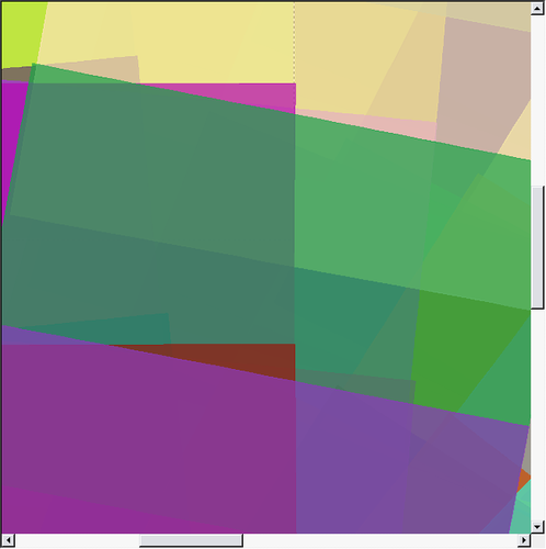
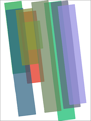
The automatic seeding program is dependent on the information about how all the images to be combined into a single output overlap each other. The polygons can be different shapes and sizes. A separate program ( findimageoverlaps ) attempts to find all the polygons and saves the information to an output file. This output file is defined as the overlap parameter in autoseed . The example below shows the overlap polygons in different shades of color.

What algorithms are available? ¶

The three algorithms available are the following:

Grid - best for different shapes and sizes of overlap polygon
Limit - use to limit the number of seeded tiepoints per polygon
Strip - best for rectangular shaped overlap polygons such as those for adjacent line scan data

The standard autoseed templates for the three algorithms are in $ISIS3DATA/base/templates/autoseed/

What are the required parameters for the different algorithms? ¶

The required parameters for each algorithm are provided through a separate Parameter Value Language (PVL) definition file.

Example of the contents of a PVL file for the grid algorithm:

Object = AutoSeed
  Group = PolygonSeederAlgorithm
    Name = Grid
    Minimum Thickness = 0.0
    MinimumArea = 100000000
    XSpacing = 10000
    YSpacing = 10000
  EndGroup
EndObject

Example of the contents of a PVL file for the limit algorithm:

Object = AutoSeed
  Group = PolygonSeederAlgorithm
    Name = Limit
    Minimum Thickness = 0.0
    MinimumArea = 100000000
    MajorAxisPoints = 6
    MinorAxisPoints = 3
  EndGroup
EndObject

Example of the contents of a PVL file for the strip algorithm:

Object = AutoSeed
  Group = PolygonSeederAlgorithm
    Name = Strip
    Minimum Thickness = 0.0
    MinimumArea = 100000000
    XSpacing = 10000
    YSpacing = 10000
  EndGroup
EndObject

Example of using keywords to specify a set of valid parameters to seed tie points:

Object = AutoSeed
  Group = PolygonSeederAlgorithm
    Name = Grid
    MinimumThickness = 0.0
    MinimumArea = 1000 <meters>
    XSpacing = 20000 <meters>
    YSpacing = 10000 <meters>
    PixelsFromEdge = 20.0
    MinEmission = 20.0
    MaxEmission = 75.0
    MinIncidence = 25.0
    MaxIncidecne = 80.0
    MinResolution = 255.0
    MaxResolution = 259.0
    # MinDN and MaxDN are costly checks
    MinDN = 0.145
    MaxDN = 0.175
  EndGroup
EndObject

What is the MinimumThickness parameter? ¶

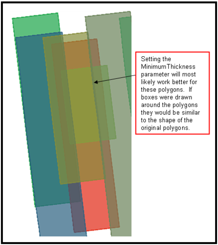
The MinimumThickness is used to exclude seeding tiepoints within polygons that are narrow slivers. If the thickness value is below the defined minimum thickness, then no tiepoints are seeded within the polygon. The valid values are between 0.0 and 1.0, and the default value is 0.0 if nothing is entered. The thickness value is derived by drawing a box around the polygon, and calculating the ratio of the short side by the long side of the box. The MinimumThickness option works best if the polygons are rectangular or square shapes. Use this parameter with caution because the calculated value for thickness may not be accurate.

What is the MinimumArea parameter? ¶

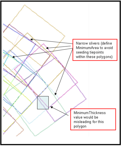
The MinimumArea is used to specify what the smallest calculated value for the minimum area of an overlap polygon must be in order to seed tiepoints. The default value is 0.0 if nothing is entered for MinimumArea. This parameter is useful for excluding small and skinny overlap polygons from being seeded with tiepoints.

What are XSpacing and YSpacing ? ¶

The grid and strip algorithms require the user to define XSpacing and YSpacing, and if nothing is entered the program will report an error and fail. The XSpacing and YSpacing parameters are defined in meters, and determine how the tiepoints will be distributed within each polygon. The tiepoints are seeded starting at the center of each polygon, and spaced every XSpacing increment along the X-axis, and YSpacing increment along the Y-axis. The resolution of the input images will contribute to how dense the tiepoints are seeded. See Examples .

What are MajorAxisPoints and MinorAxisPoints ? ¶

These two parameters are only used for the Limit algorithm. The MajorAxisPoints is used to specify how many tiepoints to seed along the longer side of a box drawn around the polygon. The MinorAxisPoints is used to specify how many tiepoints to seed along the shorter side of a box drawn around a polygon. So, if you set MajorAxisPoints = 10 and MinorAxisPoints = 3, then you would have 30 equally spaced tiepoints (10 rows by 3 columns or 3 rows by 10 columns) within each of the overlap polygons.

What programs must be run before running autoseed? ¶

The following programs must be run on individual input images:

spiceinit - attaches SPICE data to the ISIS3 cube
footprintinit - adds image footprint information to ISIS3 cube labels
camstats - attaches geometric and image statistics to the ISIS3 cube labels

The following program requires a list of images as input:

findimageoverlaps - determines all the overlap polygons among all the
   images in the input list

How do you determine which algorithm to use? ¶

The first step is to display the images you have selected to see how they overlap each other using either PILOT, qmos, or some other display method. The overlap polygons are areas where a unique set of images overlap each other. The complexity of the polygons across your mosaic area will determine which algorithm is the most appropriate to use.

Examples:

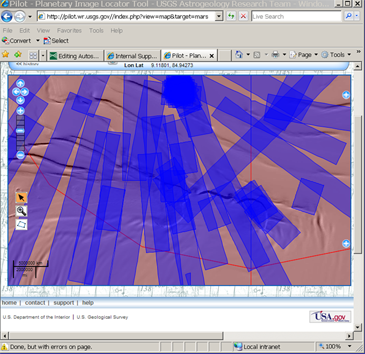
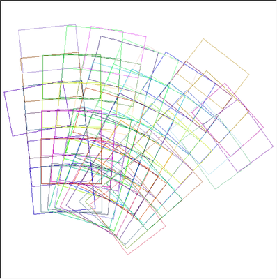
This is an example of the rendered images using Astrogeology UPC image search ( PILOT ). The image footprints are not in a uniform order, and the size of the images varies. The grid algorithm would be the best to use for this data.

In this example, the resolution of the images are about the same, but the ground area that was imaged varies in size. The strips of CTX linescan data are adjacent to each other, and the overlap polygons are simple and easily identified. The limit algorithm would be the easiest to use. You would need to decide how many points to seed along the longest side of the overlap polygon and how many points across the shorter side. The strip algorithm will provide more evenly distributed set of tiepoints, but you will need to figure out the most appropriate X and Y spacing.

In this example, the resolution of the images are about the same. The size of the overlap polygons vary in shape, orientation, and sizes. It would be best to specify the MinimumArea to eliminate many of the smaller polygons from getting seeded. The best option would be to use either grid or strip algorithm to avoid clustered points in the smaller polygons. The MinimumArea can be increased if there are too many points clustered together in the smaller polygons, and the spacing can also be increased to put a greater distance between the seeded tiepoints.

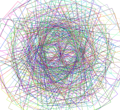
In this example, the overlap polygons are so complex that findimageoverlaps will fail, and autoseed cannot be run. In this case, the only option is to use the program seedgrid to generate a network of seeded tiepoints. The seedgrid program does not require prior knowledge of the overlap polygons, but does require latitude range, longitude range, and a map template.

How do you determine XSpacing and YSpacing? ¶

It is important to know the range of resolutions for the images you wish to include. Decide how many tiepoints you want to seed across the longer side and shorter side of the overlap polygons. For example, let’s say most of the polygons have 50 pixels of overlap along the shortest width and 5000 pixels along the longest length and the median resolution is 6 meters/pixel, and you have decided to seed 3 points across the shorter side and 10 points along the longer side of the polygons. The calculation for the spacing would be the following:

X-spacing = (50/(3 + 1)) * 6  =  75m
y-spacing = (5000/(10 + 1)) * 6 = ~2727m (round up to 2800m)

The second option is to display two images whose overlap pattern is representative of most of the images in the mosaic using ISIS3 qview program. The following is an example of the qview measurement tool, depicted as a ruler on the right side, to measure the distance of the widest overlap area:

See Using Qview to view cubes for more information about qview .

Example of measurement tool on two Clementine images to show the overlap area in meters

The tool measured approximately 278 pixels. The resolution of these two images are around 190 meters/pixel. So, the calculation for XSpacing would be ((278 pixels/6) * 190 m/pixel) resulting in 8803.3 meters. You could start with XSpacing and YSpacing equal to 8800 meters as a starting point, and then increase or decrease the number based on whether you want to increase or decrease the distance between the seeded tiepoints.

Example of measurement tool on two Clementine images to show the overlap area in meters

This example shows the measurement for the shorter side of the polygon, which is about 86 pixels. Sometimes the spacing increments you select may need to be different in the x and y directions, especially for line scan data where the image has a lot more lines than samples. If the desire is to seed only two tiepoints along the shorter side then your calculation would be ((86 pixels/3) * 190 m/pixel) giving an xspacing of 5446 meters. You could use 5500 meters for x-spacing and 8800 meters for y-spacing.

What are the required parameters for autoseed and how do you run the program? ¶

Autoseed parameters:

fromlist - list of all the filenames to be included in a control solution
deffile - PVL file containing the seeding algorithm and spacing between
          the tiepoints
overlaplist - the output file from findimageoverlaps program
cnet - if you wish to add to an existing control network file, enter the
       filename
onet - the output filename for the control network file generated by
       autoseed
errors - the output filename for error tracking for autoseed
networkid - an ID name assigned to the control network file
pointid - the starting string to be assigned to the PointId's plus
          question marks for number of digits needed, normally provided
          as "C?????"
description - provide a description of the contents of the output
              control net file

Example of the autoseed GUI interface

Example of autoseed GUI interface

The user also has the option of running the program by typing the following command line as a continuous string without using the GUI interface:

autoseed fromlist=lev1.lis deffile=clem_grid2_autoseed.def
overlaplist=overlaps.lis onet=autoseed_grid.net errors=autoseed_grid.err
networkid=Clementine1 pointid=C\?\?\?\?\?\? description="Clementine grid1"

What is the result of autoseed? ¶

The output file is a binary control network (cnet) file that contains the control pointids and control measurements of all the images that overlap each seeded tiepoint. The program qmos can be used to display the images, image footprints, and the control network to see how the tiepoints are distributed. If the distribution of tiepoints is too dense, increase the spacing between the tie points to spread them apart and to reduce the number of tiepoints. If the tiepoints are too sparse then decrease the spacing to add more tiepoints. Rerun autoseed each time the parameters in the PVL definition file are changed. When you have reached an acceptable solution then use the program qnet to evaluate and refine the tiepoints by loading the control network file.

The output network can no longer be viewed by a text editor unless the network file has been converted to a PVL format with cnetbin2pvl , but use caution if the file size is large. The second option is to use cneteditor to view the network file in the binary format.

Convert binary control network to PVL format:

cnetbin2pvl from=hirise_set1_autoseed.net to=hirise_set1_autoseed_pvl.net

Example of the contents of a HiRISE cnet file (first 66 lines):

Object = ControlNetwork
 NetworkId    = Hirise_set1
 TargetName   = Mars
 UserName     = elee
 Created      = 2012-05-08T10:38:21
 LastModified = 2012-05-08T10:38:21
 Description  = "HiRise set1 images autoseed with hirise_ccd_sets_seed.def"
 Version      = 3

 Object = ControlPoint
   PointType   = Free
   PointId     = hirise_set1_00001
   ChooserName = autoseed
   DateTime    = 2012-05-08T10:38:45

   Group = ControlMeasure
     SerialNumber  = MRO/HIRISE/867676384:40724/RED0/2
     MeasureType   = Candidate
     ChooserName   = autoseed
     DateTime      = 2012-05-08T10:38:45
     Sample        = 2040.423603891
     Line          = 20.242382897271
     AprioriSample = 2040.423603891
     AprioriLine   = 20.242382897271
   End_Group

   Group = ControlMeasure
     SerialNumber  = MRO/HIRISE/867676384:40724/RED1/2
     MeasureType   = Candidate
     ChooserName   = autoseed
     DateTime      = 2012-05-08T10:38:45
     Sample        = 43.186441092459
     Line          = 13.357872143126
     AprioriSample = 43.186441092459
     AprioriLine   = 13.357872143126
   End_Group
 End_Object

 Object = ControlPoint
   PointType   = Free
   PointId     = hirise_set1_00002
   ChooserName = autoseed
   DateTime    = 2012-05-08T10:38:45

   Group = ControlMeasure
     SerialNumber  = MRO/HIRISE/867676384:40724/RED0/2
     MeasureType   = Candidate
     ChooserName   = autoseed
     DateTime      = 2012-05-08T10:38:45
     Sample        = 2011.1452341621
     Line          = 16.380977898313
     AprioriSample = 2011.1452341621
     AprioriLine   = 16.380977898313
   End_Group

   Group = ControlMeasure
     SerialNumber  = MRO/HIRISE/867676384:40724/RED1/2
     MeasureType   = Candidate
     ChooserName   = autoseed
     DateTime      = 2012-05-08T10:38:45
     Sample        = 13.917053834296
     Line          = 9.5400377909342
     AprioriSample = 13.917053834296
     AprioriLine   = 9.5400377909342
   End_Group
 End_Object

Display the control network with cneteditor:

cneteditor hirise_set1_autoseed.net

Example of a partial listing of a control network file using cneteditor

The example above shows a snapshot of the cneteditor GUI. The window can be expanded to see additional columns.

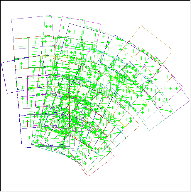
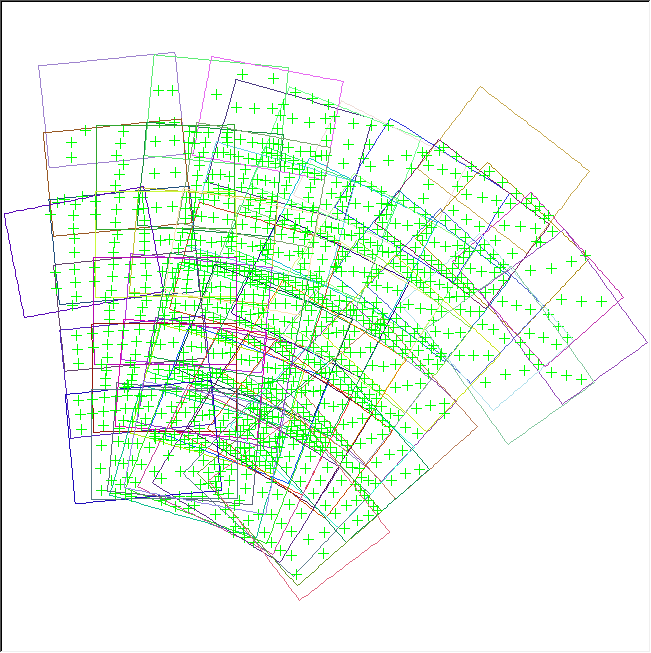
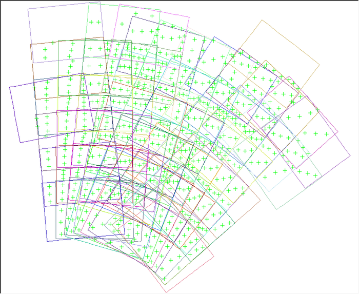
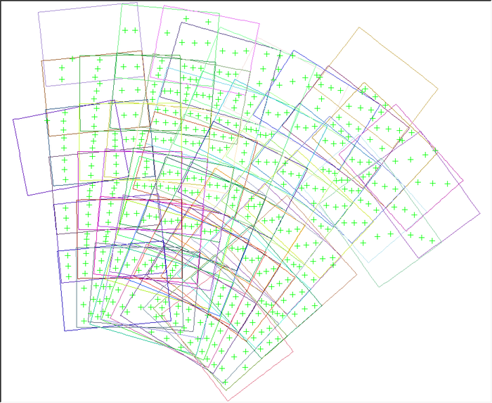
Examples of image footprint and tiepoints plotted with different parameter settings. ¶

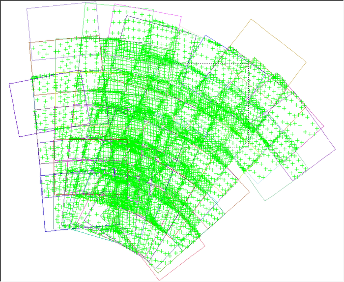
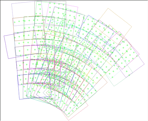
Coarse grid example ¶


Autoseed automatically seeded tiepoints for Clementine images

Autoseed PVL definition file for Grid alogrithm

Name = Grid
MinimumThickness = 0.0
MinimumArea = 10000000
XSpacing = 10000
YSpacing = 10000

The spacing increment for both X and Y directions are the same due to the similar shapes of the overlap polygons. The MinimumArea was defined to limit clustered tiepoints.

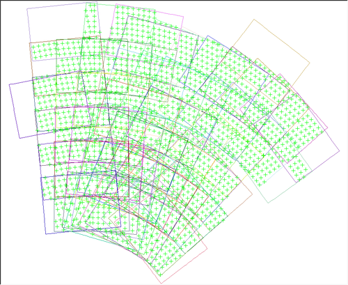
Fine grid example ¶


Autoseed automatically seeded tiepoints for Clementine images

Autoseed PVL definition file for Grid algorithm

Name = Grid
MinimumThickness = 0.0
MinimumArea = 10000000
XSpacing = 5000
YSpacing = 5000

The spacing increment decreased by a factor of two so more tiepoints can be automatically seeded. It was desirable to have more tiepoints due to the fact that we are working with data near the South Pole where there are more areas in shadows than normal.

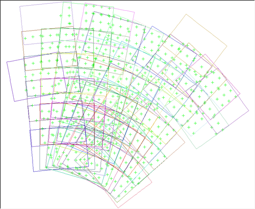
Coarse strip example ¶


Autoseed automatically seeded tiepoints for Clementine images

Autoseed PVL definition file for Strip alogrithm

Name = Strip
MinimumThickness = 0.0
MinimumArea = 10000000
XSpacing = 10000
YSpacing = 10000

The spacing increment for both X and Y directions are the same due to the similar shapes of the overlap polygons. The MinimumArea was defined to limit clustered tiepoints. The result is very similar to the grid algorithm and some of the tiepoints are seeded in difference locations.

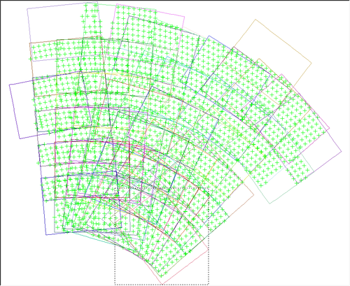
Fine strip example ¶


Autoseed automatically seeded tiepoints for Clementine images

Autoseed PVL definition file for Strip alogrithm

Name = Strip
MinimumThickness = 0.0
MinimumArea = 10000000
XSpacing = 5000
YSpacing = 5000

The spacing increment decreased by a factor of two so more tiepoints can be automatically seeded. It was desirable to have more tiepoints due to the fact that we are working with data near the South Pole where there are more areas in shadows than normal. There are more tiepoints clustered along polygon boundaries for this test.

Limit example ¶

Starting Point ¶

MinimumThickness = 0.0
MinimumArea = 10000000
MajorAxisPoints = 6
MinorAxisPoints = 3

The starting point.

Step 1 ¶

MinimumThickness = 0.0
MinimumArea = 10000000
MajorAxisPoints = 3
MinorAxisPoints = 1

The number of points for the major and minor axis were reduced to seed fewer tiepoints.

Step 2 ¶

MinimumThickness = 0.0
MinimumArea = 20000000
MajorAxisPoints = 3
MinorAxisPoints = 1

The MinimumArea was doubled to eliminate tiepoints in the small polygons.

Step 3 ¶

MinimumThickness = 0.0
MinimumArea = 50000000
MajorAxisPoints = 3
MinorAxisPoints = 1

The MinimumArea was increased again to remove more tiepoints from the small polygons.

Step 4 ¶

MinimumThickness = 0.0
MinimumArea = 75000000
MajorAxisPoints = 3
MinorAxisPoints = 1

The MinimumArea was increased even further to eliminate tiepoints that were still too close together especially along the polygon boundaries.

What is seedgrid ? ¶

The last option is to utilize seedgrid instead of autoseed if findimageoverlaps fails. This method seeds tiepoints without relying on the overlap polygons. The program will seed tiepoints across a specified area based solely on the spacing provided by the user, either in x/y spacing or lat/lon increment. The output file will contain the PointId and the latitude and longitude coordinate associated with each pointid. This option is also useful if your data set includes images with a wide range of resolutions, or if the limb or terminator in the image.

Example of running seedgrid as a command line: ¶

seedgrid target=Mars minlat=0 maxlat=5 minlon=0 maxlon=6
spacing=latlon latstep=1 lonstep=1 networkid=Seedgrid1
pointid=Mars_seedgrid_\?\?\? onet=seedgrid.net
description="Seedgrid latinc=1 loninc=1"

cnetbin2pvl from=seedgrid.net to=seedgrid_pvl.net

Partial contents of seedgrid control network file:

Object = ControlNetwork
 NetworkId    = Seedgrid1
 TargetName   = Mars
 UserName     = elee
 Created      = 2012-06-01T11:07:49
 LastModified = 2012-06-01T11:07:49
 Description  = "Seedgrid latinc=1 loninc=1"
 Version      = 3

 Object = ControlPoint
   PointType   = Free
   PointId     = Mars_seedgrid_001
   ChooserName = seedgrid
   DateTime    = 2012-06-01T11:07:49
   Ignore      = True

   # AprioriLatitude = 0.0 <degrees>
   AprioriX    = 3396190.0 <meters>

   # AprioriLongitude = 0.0 <degrees>
   AprioriY    = 0.0 <meters>

   # AprioriRadius = 3396190.0 <meters>
   AprioriZ    = 0.0 <meters>
 End_Object

 Object = ControlPoint
   PointType   = Free
   PointId     = Mars_seedgrid_002
   ChooserName = seedgrid
   DateTime    = 2012-06-01T11:07:49
   Ignore      = True

   # AprioriLatitude = 1.0 <degrees>
   AprioriX    = 3395672.7438132 <meters>

   # AprioriLongitude = 0.0 <degrees>
   AprioriY    = 0.0 <meters>

   # AprioriRadius = 3396190.0 <meters>
   AprioriZ    = 59271.688218238 <meters>
 End_Object

The next step would be to run cnetadd to add new control measurement for the images in your input list.

ls *lev1.cub > lev1.lis
cnetadd cnet=seedgrid.net addlist=lev1.lis onet=seedgrid_cnetadd.net
tolist=cnetadd_output.lis log=seedgrid_cnetadd.log modifiedpoints=modified.lis
polygon=yes retrieval=point

Continue with control registration with pointreg or other cnet programs.

Autoseed_gui_2012.png View (79.3 KB) Jesse Mapel, 2016-05-31 12:58 PM

Clem_grid1_autoseed.png View (83.8 KB) Jesse Mapel, 2016-05-31 12:58 PM

Clem_grid2_autoseed.png View (104 KB) Jesse Mapel, 2016-05-31 12:58 PM

Clem_footprint_plot.png View (141 KB) Jesse Mapel, 2016-05-31 12:58 PM

Clem_limit1_autoseed.png View (115 KB) Jesse Mapel, 2016-05-31 12:58 PM

Clem_limit3_autoseed.png View (67.7 KB) Jesse Mapel, 2016-05-31 12:58 PM

Clem_limit2_autoseed.png View (68.7 KB) Jesse Mapel, 2016-05-31 12:58 PM

Clem_limit4_autoseed.png View (82.4 KB) Jesse Mapel, 2016-05-31 12:58 PM

Clem_polar_footprints.png View (148 KB) Jesse Mapel, 2016-05-31 12:58 PM

Clem_strip1_autoseed.png View (82.6 KB) Jesse Mapel, 2016-05-31 12:58 PM

Clem_strip2_autoseed.png View (108 KB) Jesse Mapel, 2016-05-31 01:00 PM

Cneteditor_2012.png View (77.5 KB) Jesse Mapel, 2016-05-31 01:00 PM

Ctx_footprint_plot.png View (114 KB) Jesse Mapel, 2016-05-31 01:00 PM

Ctx_footprint_plot_cropped_demo.png View (47 KB) Jesse Mapel, 2016-05-31 01:00 PM

Overlap_polygon_example.png View (22.9 KB) Jesse Mapel, 2016-05-31 01:00 PM

Narrow_sliver_polygon_example.png View (84.4 KB) Jesse Mapel, 2016-05-31 01:00 PM

Qview_measure_for_spacing_calculation_indexcolor.png View (94.5 KB) Jesse Mapel, 2016-05-31 01:00 PM

Qview_moreoverlap_measure_for_spacing_calculationt.png View (126 KB) Jesse Mapel, 2016-05-31 01:00 PM

UPC_CTX_search_for_footprint_reduced.png View (170 KB) Jesse Mapel, 2016-05-31 01:00 PM

Clem_limit5_autoseed.png View (79 KB) Jesse Mapel, 2016-05-31 02:25 PM